Phase II Envelope Iteration: Mk1 -> Mk2 -> Mk3 (Aerodynamics Focus)

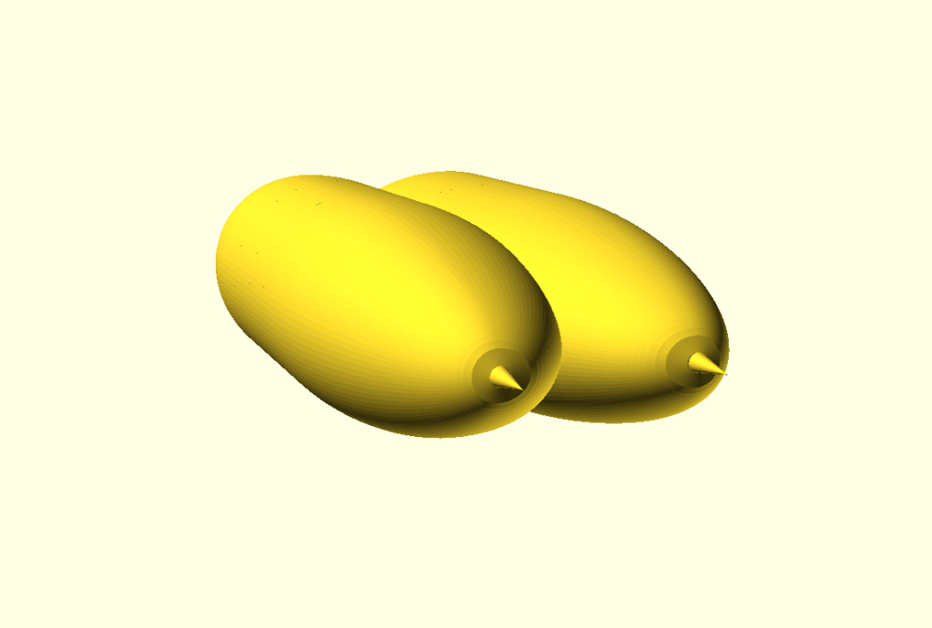
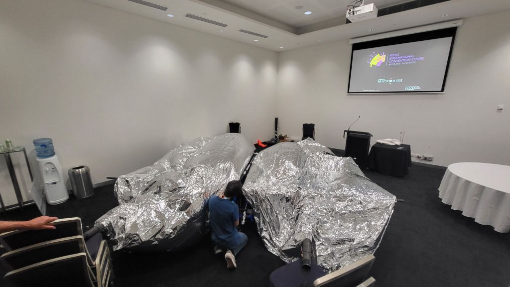
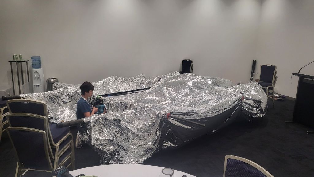
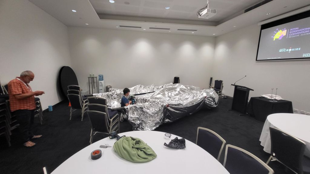
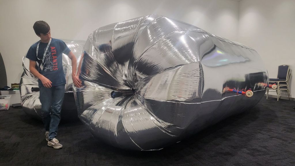
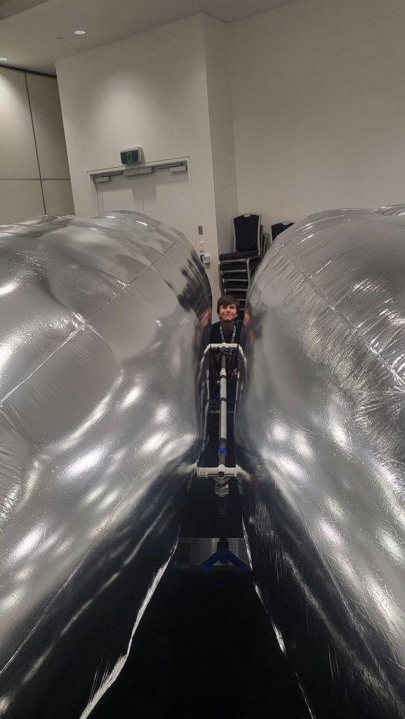
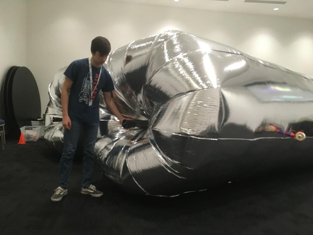
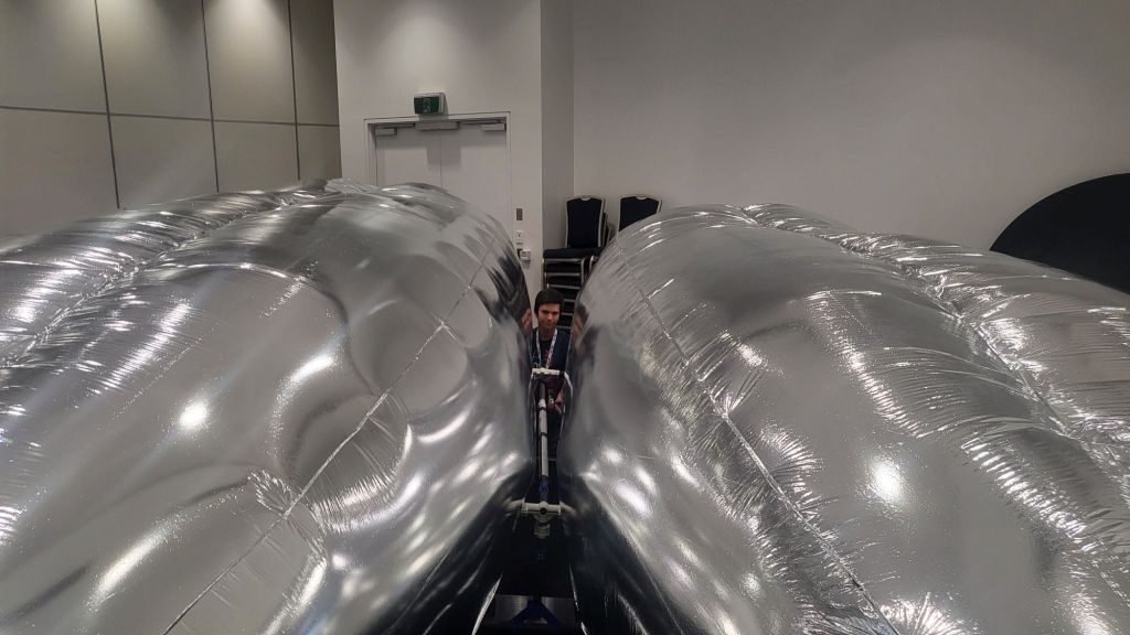
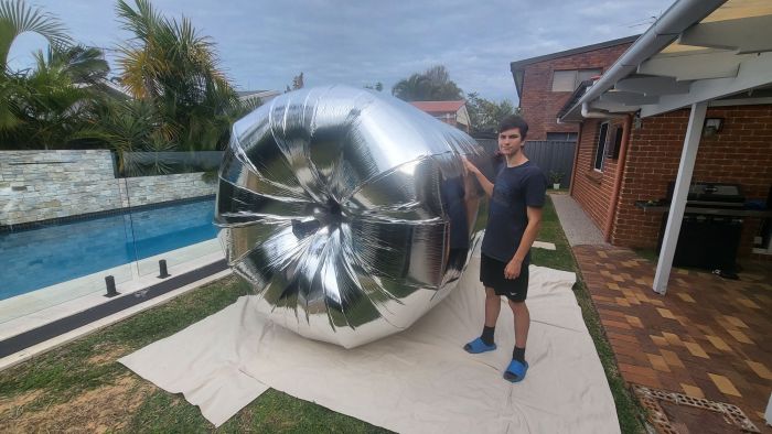
As part of our Phase II envelope design, we wanted to understand how the interface between two adjacent hulls affects turbulence and parasitic drag.

Mk1, Mk2 and Mk3 variants were developed to explore how these envelope shapes behave within the CFD (Computer Fluid Dynamics) modelling

The short version:

  • Mk1 gave us a clean baseline
  • Mk2 reduced the deep center cleavage effect by reshaping the lobe interaction.
  • Mk3 removed cleavage entirely (convex hulled pair) to test the upper bound of this effect.

Design Workflow

For each iteration, we:
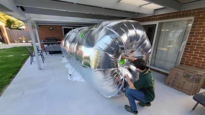
1. Modelled geometry in OpenSCAD (src/scad/phase2_envelope_cli.scad).
2. Exported STL in a binary format.
3. Ran a FluidX3D single continuous sweep (0 -> 50 -> 0 km/h) with drag recording.
4. Produced visual overlays (3840×2160) and drag timeseries for comparison.

Common Baseline Parameters

These were the shared baseline values for this iteration cycle:

  • length_mm=19000 //overall length
  • diameter_mm=5000 //maximum diameter
  • nose_len_mm=4500 //front gasbag length
  • cyl_len_mm=6000 //central gasbag length
  • tail_len_mm=8500 //tail gasbag length
  • hull_spacing_mm=4000
  • keel_tube_inner_diameter_mm=400
  • $fn=200 //OpenSCAD rendering resolution

CFD sweep profile baseline:

  • single sweep mode (0 -> 10 -> 20 -> 30 -> 40 -> 50 -> … -> 0)
  • ramp: 3s
  • hold: 5s
  • total run: 80s
  • drag timeseries exported to drag_timeseries.csv

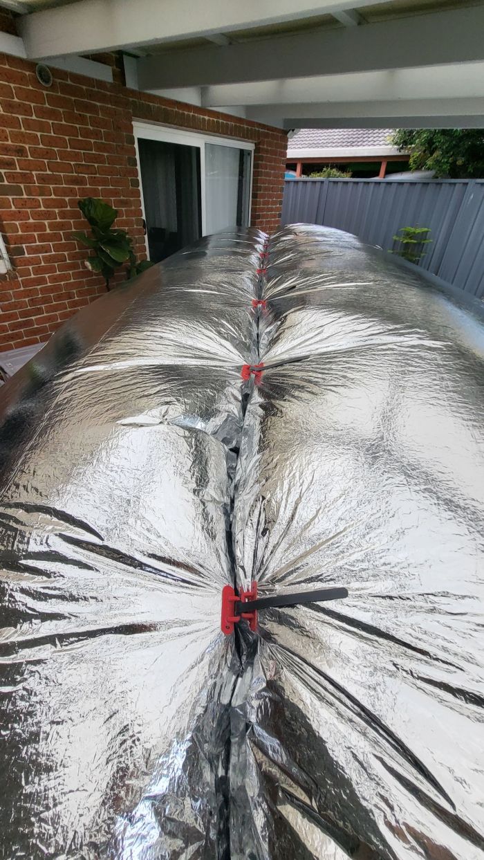
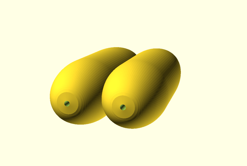
Mk1 (Legacy Overlap)

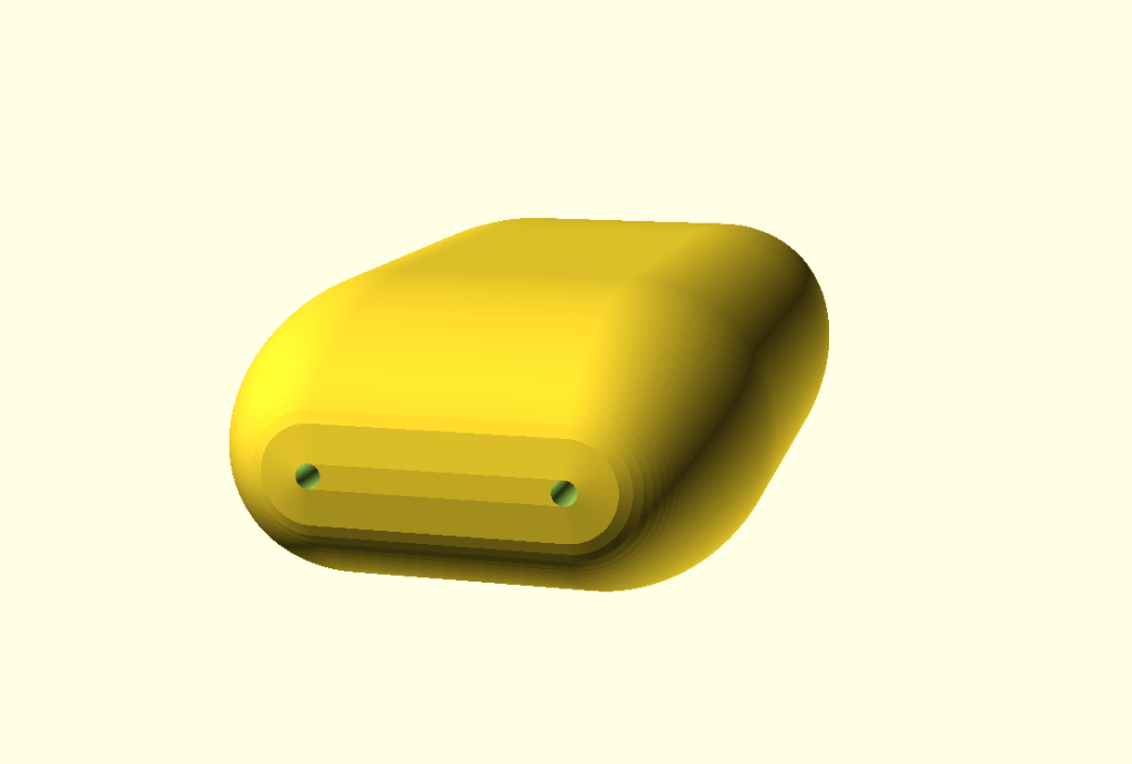
Mk1 gave us a clean baseline – Formed by two circular-section envelopes in legacy overlap arrangement.

FluidX3D run output:

Observation summary:

  • Clear center-interface turbulence (deep cleavage behavior) was visible in wake dynamics.
  • Max |drag_N|: 7129 N (at 50 km/h)

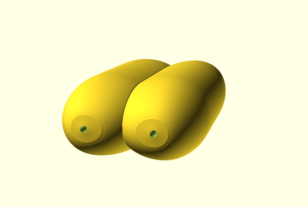
Mk2 (Bulged Bell Interaction)

In this iteration we replaced circular interaction with bell-like lobe shaping to emulate how envelopes may lean/bulge into each other.

Key shaping controls:

  • lobe_profile_mode=”bell”
  • bulge_strength=0.18
  • max_lobe_squeeze=0.28
  • bell_flare=0.45
  • bell_base_gap_mm=0
  • bell_smoothing_mm=100
  • bell_inner_scale=1.3

FluidX3D run output:

Observation summary:

  • Substantial visible improvement in center-interface flow behavior vs Mk1.
  • Max |drag_N|: 7316 N (at 50 km/h)

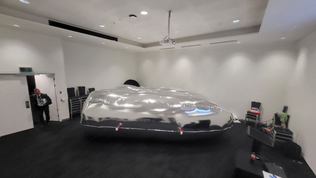
Mk3 (Hulled Pair / Cleavage Removed)

In this iteration convex hull across both envelopes was to eliminate cleavage entirely and test how strongly it drives losses.

FluidX3D run output:

Observation summary:

  • Intended as a limit-case experiment to quantify how much center-cleavage geometry dominates drag/turbulence.
  • Max |drag_N|: 8040 N (at 50 km/h)

Drag Comparison (Parasitic Drag Evaluation)

Then we compared drag values from the continuous sweep windows across all three marks.

Windowed hold means (drag_N) from corrected controlled rerun (values in a table are from a low-res run where they ended up being ~10% higher potentially due to the model resolution):

WindowMk1 mean drag (N)Mk2 mean drag (N)Mk3 mean drag (N)Mk2 vs Mk1Mk3 vs Mk1Mk3 vs Mk2
10_up484.1512.7570.2+5.92%+17.78%+11.20%
20_up1612.31720.91895.2+6.74%+17.54%+10.12%
30_up3327.93556.03828.9+6.85%+15.05%+7.68%
40_up5510.95777.36251.8+4.83%+13.44%+8.21%
50_up8016.68375.38995.5+4.48%+12.21%+7.40%
40_down5499.15787.96307.5+5.25%+14.70%+8.98%
30_down3344.63558.83896.1+6.40%+16.49%+9.48%
20_down1580.31724.91877.9+9.15%+18.83%+8.88%
10_down415.5465.1486.1+11.94%+16.97%+4.50%

Overall hold-window mean:

  • Mk1: 3316.88 N (best)
  • Mk2: 3504.64 N (+5.66% vs Mk1)
  • Mk3: 3797.41 N (+14.48% vs Mk1, +8.35% vs Mk2)

Decision under current assumptions:

  • Mk1 is the lowest-drag geometry in this controlled batch.
  • Mk2 and Mk3 visibly alter center-flow structure, but in this setup those changes did not reduce integrated parasitic drag.
  • The comparison plot artifact is at out/fluidx_phase2_runs/phase2_controlled_mk_compare_20260215_223154/drag_compare_plot_absN.png. [TBA]

AWS rerun status note (February 24, 2026):

  • We started a fresh Mk3 AWS rerun after fixing headless render sizing.
  • This rerun is intended as infrastructure/throughput validation plus additional data for later cross-hardware comparison (not yet replacing the corrected local controlled ranking above).

Compute platform snapshot used in this phase:

  • Local runs were executed on a workstation with NVIDIA GeForce RTX 4060 (8188 MiB VRAM observed).
  • AWS test path started on g6f.large (fractional L4, ~3 GiB VRAM) and then moved to g6.8xlarge (full L4, 23034 MiB VRAM observed).
  • On g6.8xlarge with the current upper-edge settings, measured throughput projects roughly:
    • ~20.5h for one full single sweep (SECS=80)
    • ~61h for three sequential sweeps at the same settings

This confirms the aerodynamic ranking table above should still rely on the corrected controlled local batch for decision-making today. AWS high-VRAM runs are currently most valuable for higher-resolution validation and hardware scaling evidence.

Infrastructure planning note:

In this run shape, one sweep process occupies one GPU, so the best cost/performance default is typically a 1x-L4 instance (g6.xlarge) rather than larger 1x-L4 sizes. Larger L4 instances are still useful when we need more CPU/RAM headroom, but not as default for single-process CFD throughput.

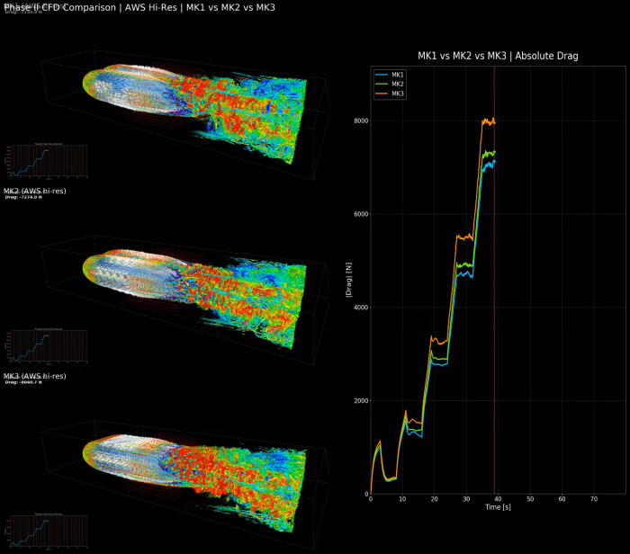
Final Consolidated Update (AWS Hi-Res, March 1, 2026)

We now have the full Mk1/Mk2/Mk3 AWS high-resolution set consolidated and compared in one place + comparison bundle.

AWS hi-res hold-window means (drag_N) confirm the same ordering:

  • Mk1: `2810.15 N` (best)
  • Mk2: `2940.53 N` (`+4.64%` vs Mk1)
  • Mk3: `3257.12 N` (`+15.91%` vs Mk1, `+10.77%` vs Mk2)

Cross-platform consistency note:

  • Local low-res and AWS hi-res are consistent in ranking/trend, but not interchangeable in absolute magnitude.
  • Hi-res/low-res drag scale averaged about 0.81x (Mk1 0.817, Mk2 0.808, Mk3 0.816).

40 km/h engineering point (AWS hi-res):

  • Mk1: 4704.71 N -> aerodynamic power 52.27 kW
  • Mk2: 4905.22 N -> aerodynamic power 54.50 kW
  • Mk3: 5485.55 N -> aerodynamic power 60.95 kW

Volume-normalized interpretation at 40 km/h:

  • Mk1 volume: 552.022 m^3, 8.52 N/m^3
  • Mk2 volume: 577.873 m^3, 8.49 N/m^3 (slightly best per volume)
  • Mk3 volume: 608.412 m^3, 9.02 N/m^3

Mk2 Local Tail/Fineness Optimization Check (March 1, 2026)

To test if small Mk2 shape changes can materially reduce cruise drag, we ran a focused local optimization batch:

  • run: phase2_mk2_opt40_batch1_calconly_patched4_20260301_203453
  • objective protocol: 0 -> 40 -> 0 km/h (ramp=2s, hold=4s)
  • score: mean |drag_N| in [t=3s, t=5s]
  • volume guardrail: keep at/above Mk2 baseline volume

Best candidate in this batch worked out to be “c010_tl9000_tb0p45” coming with drag@40: 5584.71 N. This local neighbourhood did not produce a better-than-Mk2 design so for current Phase II decision-making, Mk2 remains the practical baseline as expected envelope-only savings from further incremental shape tuning are likely modest unless a stronger new geometry concept is introduced.

So here is our winner – Mk2 reduced the deep center cleavage!

Envelope wedge clamps – green

In continuation of our work on envelope fixes, we repeated all the steps from last weekend with the starboard “green” envelope.

Knowing what we are up to, all job went much smoother this time. Inflated envelope seemed to be holding pressure in an acceptable manner.

After making significant progress with our initial milestones, our focus shifted to one last problematic component: the central gondola tube. This particular tube had suffered multiple fractures during previous test runs.

The failures were traced to excessive torsional forces acting on the tube. As the central gondola tube connects directly to the main traverse tubes (each 4 meters long and spaced 2 meters apart through the envelopes), it experienced substantial torsional loading from these points of attachment.

The diagram above illustrates the torsional stress distribution on a cylindrical element. The twisting action creates uneven shear stresses, which the initial central tube design wasn’t adequately prepared to withstand. In hindsight, we’re fortunate that the damage was confined to this tube, preventing a more systemic failure that could have propagated through the entire structure.

After discussing this with Serge, we decided on an alternative solution, which is depicted below.

The new design involves a split aluminum tube at the center, with an additional overlapping section designed to transfer all loads except torsional forces. The aluminum tube is shielded by a rubber hose, which is clamped at both ends using hose clamps. This rubber overlay allows for some controlled torsion flexibility, effectively acting as a damper to reduce stress concentrations. The intent behind this assembly is to isolate and minimize torsional forces on the main central tube, while still allowing the structure to behave elastically and return to its original state post-deformation.

This redesign should improve the resilience of the central tube, reducing the risk of fracture during future test flights and ensuring the gondola’s stability under dynamic conditions.

Obviously replacing super-light CF tube with Aluminum one came with a cost. Weighing revealed that gondola structure is now ~700g heavier. With the excess of 10kg we measured last time it shouldn’t be a big deal and I hope that this investment will pay off.

And that’s it for last weekend! Stay tuned as we are planning all motors test next week!

Envelope wedge clamps – red

As nearing to our first motorised flight, there are/were still few things to take care of. Probably the one most pressing was the way how the envelope upper wedge was clamped, where using the Ametalin tape shown to be unreliable (tape was ripping off as envelope inflated).

Ametalin tape used to clamp the envelope wedge

Anyway, so designed new clamp in OpenSCAD which goes through the envelope and provides means to strap both sides together while distributing the load in some convenient way (Eye foundation is 30 degrees bent). Code is pretty simple:

use <ShortCuts.scad>

$fn=100;

module joint(angleIn) {
rotate_extrude(angle = angleIn)
translate([3,0,0])
circle(3);
}

module clamp() {
Ty(13)
cylinder(10, 3, 3);
T(-3,13,0)
R(90,30,0)
joint(30);
Ry(30)
T(0.4,13,-4.5)
cylinder(3, 2, 3);

Ty(-13)
cylinder(10, 3, 3);
T(-3,-13,0)
R(90,30,0)
joint(30);
Ry(30)
T(0.4,-13,-4.5)
cylinder(3, 2, 3);

T(0, 10, 13)
Rx(90)
cylinder(20, 3, 3);

T(0,10,10)
Ry(-90)
joint(90);

T(0,-10,10)
R(0,-90,180)
joint(90);
}

module pads(upper = true) {
D() {
if (upper) {
minkowski() {
cube([1.5,40,0.01], center = true);
cylinder(1.5,10,10);
}
}else{
Tz(-1.5)
minkowski() {
cube([1.5,40,0.01], center = true);
cylinder(1.5,10,10);
}}
T(0.4,-13,-1.55)
cylinder(3.1, 2.05, 3.05);

T(0.4,13,-1.55)
cylinder(3.1, 2.05, 3.05);
}}

module pegs() {
Tz(-0.1)
cylinder(1.1,1,1);
Tz(1)
sphere(1);

T(0,22,-.1)
cylinder(1.1,1,1);
T(0,22,1)
sphere(1);

T(0,-22,-0.1)
cylinder(1.1,1,1);
T(0,-22,1)
sphere(1);
}

clamp();

*pads(false);
*pegs();

D() {
pads(true);
pegs();
}

Resulting rendering:

Now, printed all parts many times (each side of wedge has those distributed every 50 cm + multiplied twice for each envelope). Then lots of gluing and it worked out very well – see our weekend inflation test which demonstrates that that idea works pretty well.

Another part installed was envelope gas relieve vent as deflating envelope through the maintenance opening didn’t work out well.

Installed valves actually brought a nice opportunity to see our envelope from inside for a first time showing some nice details.

Inner sleeve installation for tubes traversing envelope. Black spots on the right side are inflation valve (the big one) and pressure control valve.
Look in a forward direction, showing the intake bending & inner part of the wedge clamp (red thing all the way up)

Finally we did another inflation test which worked out in envelope bursting out in the front and around one meter long rip through it. Luckily it was anticipated that something like this can happen and we were able to fix quickly with a new weld. Inflated envelope then seemed to be keeping its shape for ~10 minutes without any signs of deflation and we took some nice pictures.

Having the port-side envelope done, the next step is to repeat all this for the starboard one, but that’s for another day. 😉

Big envelopes inflation test

Having a good go over the Hydrogen Summit 2024, I decided to do another complete assembly test back at the base, mainly to get some nice pictures for our next step.

Apparently I’ve picked hottest day in Queensland’s winter (33C) and not just that, it’s been pretty windy as well. Huge thanks to Kristian that he made himself available and came to help! Thanks to him we did some more work on envelope, mainly as those envelope openings / sleeves were not being satisfactory and also cut main tubes to their final lengths.

Then, when inflated, we took it out to our cul-de-sac to take few pictures.

I also did a 360 video myself:

I think it looks awesome! Still few things missing:

  • Tape closing the upper wedges is not sticking properly and needs some different idea on how to make it working
  • The envelope openings are not sealed properly and I don’t like that system in general. That clearly needs replacing with something clever
  • Intakes needs to be redesigned and printed again.

Finally, Seb did an awesome video with his DJI Mini 4 drone. If you’ll watch it long enough you’ll see how we’ve been transporting whole airship back to our carport.

As usual, huge thanks to a whole team, mainly to Kristian who spent practically whole Saturday putting this together and then back in pieces, Seb for his assistance & video, then Oli, Xavier and “a guy in red shorts” who made sure our airship haven’t flown away! 😀

Hydrogen Summit 2024

It’s been already 2 years since we attended Hydrogen Connect Summit Brisbane so we tried and got picked again this year!

It’s been a great opportunity for us to attempt to go for a first ever full assembly with both envelopes and it worked out great – Introducing team HyUse – Jan, Seb & Serge!

We’ve setup a nice stall to welcome whoever is interested, having all important things with us.

It took roughly 4 hours to put things together and inflate both envelopes.

It looked massive when having both envelopes fully inflated – practically filling whole meeting room!

Finally we had an opportunity to present our project to a group of VIPs. 🙂

Huge thanks to Serge & Seb & whole HyUse team! It wouldn’t be possible without you!

First inflation test

We had a great & busy weekend. Let’s let images to do the talking first.

As you can see, our project is getting from being decent to a massive fast. This is just a left envelope, while second is in the development. It took about an hour to inflate and with prevailing winds it felt like being alive (watch video below).

It was overall very satisfying feeling to see envelope’s shape for a first time. There are few deficiencies (found one insufficient welding in a rear part and slenderness of the front part can be better), but hey, its just prototype. 🙂

There are still envelope beans openings missing, main duct needs to be adjusted on its length and potentially some filler material needs to be put in to set it in properly a wedge’s centre, filling valve and pressure monitoring opening needs to be mounted … and all that once more on the other side (25% envelope welding done by now). The plan is to have it all ready to go in next two weeks, while planning for another test next weekend!

Darn centroids!

Needing to find where to put holes in an envelope we needed to find its centre of gravity first. Surprisingly there is a term for that already – a centroid! Well I’ve been lazy and explained all that to ChatGPT and it actually came back with a very sensible set of answers which I compiled into following.

Image showing a traverse truss with jigs for passing through the envelope.

Finding the Centroid of a Composite Shape: Half-Ellipses and a Rectangle

In this post, we’ll explore how to find the centroid of a composite shape made up of two half-ellipses and a rectangle. This process involves both analytical and graphical methods to ensure accuracy and clarity.

Step 1: Centroid of a Half-Ellipse

For a half-ellipse with the semi-major axis aaa and semi-minor axis bbb, the centroid (xˉ,yˉ)(\bar{x}, \bar{y})(xˉ,yˉ​) is given by:

  • xˉ=0\bar{x} = 0xˉ=0
  • yˉ=4b3Ï€\bar{y} = \frac{4b}{3\pi}yˉ​=3Ï€4b​

Step 2: Centroid Calculation for Given Shapes

Given two half-ellipses:

  • First half-ellipse with a=−3a = -3a=−3 and b=1b = 1b=1
  • Second half-ellipse with a=1.5a = 1.5a=1.5 and b=1b = 1b=1, centered at (2,0)(2,0)(2,0)

For a horizontally sliced half-ellipse:

  • First half-ellipse centroid: (0,43Ï€)(0, \frac{4}{3\pi})(0,3Ï€4​)
  • Second half-ellipse centroid: (2,4×13Ï€)(2, \frac{4 \times 1}{3\pi})(2,3Ï€4×1​)

Step 3: Centroid of a Rectangle

For a rectangle with coordinates starting at (0,−1)(0, -1)(0,−1) and ending at (2,1)(2, 1)(2,1):

  • Centroid: (xˉ3,yˉ3)=(0+22,−1+12)=(1,0)(\bar{x}_3, \bar{y}_3) = \left(\frac{0 + 2}{2}, \frac{-1 + 1}{2}\right) = (1, 0)(xˉ3​,yˉ​3​)=(20+2​,2−1+1​)=(1,0)

Step 4: Composite Shape and Its Centroid

To find the centroid of the composite shape consisting of the two half-ellipses and the rectangle:

  1. Calculate the areas (weights) of each shape:
    • Half-Ellipse 1: A1=12π×3×1=3Ï€2A_1 = \frac{1}{2} \pi \times 3 \times 1 = \frac{3\pi}{2}A1​=21​π×3×1=23π​
    • Half-Ellipse 2: A2=12π×1.5×1=1.5Ï€2=0.75Ï€A_2 = \frac{1}{2} \pi \times 1.5 \times 1 = \frac{1.5\pi}{2} = 0.75\piA2​=21​π×1.5×1=21.5π​=0.75Ï€
    • Rectangle: A3=2×2=4A_3 = 2 \times 2 = 4A3​=2×2=4
  2. Find the centroids of each shape:
    • Half-Ellipse 1: (xˉ1,yˉ1)=(−4Ï€,0)(\bar{x}_1, \bar{y}_1) = \left(\frac{-4}{\pi}, 0\right)(xˉ1​,yˉ​1​)=(π−4​,0)
    • Half-Ellipse 2: (xˉ2,yˉ2)=(2+2Ï€,0)(\bar{x}_2, \bar{y}_2) = \left(2 + \frac{2}{\pi}, 0\right)(xˉ2​,yˉ​2​)=(2+Ï€2​,0)
    • Rectangle: (xˉ3,yˉ3)=(1,0)(\bar{x}_3, \bar{y}_3) = (1, 0)(xˉ3​,yˉ​3​)=(1,0)
  3. Compute the weighted average of the centroids:
    • Total area: A1+A2+A3=3Ï€2+0.75Ï€+4=9Ï€4+4A_1 + A_2 + A_3 = \frac{3\pi}{2} + 0.75\pi + 4 = \frac{9\pi}{4} + 4A1​+A2​+A3​=23π​+0.75Ï€+4=49π​+4
    • Centroid of the composite shape: xˉ=A1â‹…xˉ1+A2â‹…xˉ2+A3â‹…xˉ3A1+A2+A3=3Ï€2⋅−4Ï€+0.75π⋅(2+2Ï€)+4â‹…19Ï€4+4≈0.3806\bar{x} = \frac{A_1 \cdot \bar{x}_1 + A_2 \cdot \bar{x}_2 + A_3 \cdot \bar{x}_3}{A_1 + A_2 + A_3} = \frac{\frac{3\pi}{2} \cdot \frac{-4}{\pi} + 0.75\pi \cdot \left(2 + \frac{2}{\pi}\right) + 4 \cdot 1}{\frac{9\pi}{4} + 4} \approx 0.3806xˉ=A1​+A2​+A3​A1​⋅xˉ1​+A2​⋅xˉ2​+A3​⋅xˉ3​​=49π​+423π​⋅π−4​+0.75π⋅(2+Ï€2​)+4â‹…1​≈0.3806
    • yˉ=0\bar{y} = 0yˉ​=0

Visualization

Below is the graphical representation of the composite shape along with the calculated centroid and cut points.

import matplotlib.pyplot as plt
import numpy as np

# Weights and centroids
W1 = 12.57
W2 = 6.0
d = 6 / np.pi + 2

# Coordinates of centroids
x1, y1 = 0, 0
x2, y2 = d, 0

# Centroid of composite shape
bar_x = 0.3806
bar_y = 0

# Points A and B
point_A = (-0.6194, 0)
point_B = (1.3806, 0)

# Define rectangle
rect_x = [0, 2, 2, 0, 0]
rect_y = [-1, -1, 1, 1, -1]

# Plot the shapes and points
plt.figure(figsize=(10, 6))

# Half-ellipses
theta = np.linspace(-np.pi/2, np.pi/2, 100)
x1 = 3 * np.cos(theta)
y1 = 1 * np.sin(theta)
x2 = 1.5 * np.cos(theta)
y2 = 1 * np.sin(theta)
cx1, cy1 = 0, 0
cx2, cy2 = 2, 0
plt.plot(cx1 - x1, cy1 + y1, label='Half-Ellipse 1 (a=-3, b=1)', color='blue')
plt.plot(cx2 + x2, cy2 + y2, label='Half-Ellipse 2 (a=1.5, b=1)', color='green')

# Rectangle
plt.plot(rect_x, rect_y, label='Rectangle', color='red')

# Centroid
plt.scatter(bar_x, bar_y, color='purple')
plt.text(bar_x, bar_y, 'Centroid', fontsize=12, ha='right', color='purple')

# Points A and B
plt.scatter(point_A[0], point_A[1], color='orange')
plt.text(point_A[0], point_A[1], 'Point A', fontsize=12, ha='right', color='orange')
plt.scatter(point_B[0], point_B[1], color='orange')
plt.text(point_B[0], point_B[1], 'Point B', fontsize=12, ha='right', color='orange')

# Formatting
plt.xlim(-4, 4)
plt.ylim(-1.5, 2)
plt.axhline(0, color='black', linewidth=0.5)
plt.axvline(0, color='black', linewidth=0.5)
plt.grid(color='gray', linestyle='--', linewidth=0.5)
plt.xlabel('X-axis')
plt.ylabel('Y-axis')
plt.title('Graph of Two Half-Ellipses with a Rectangle, Centroid, and Cut Points')
plt.legend()
plt.show()

This Python code generates the visual representation of the two half-ellipses, the rectangle, the calculated centroid, and the cut points. It ensures the correct understanding of the composite shape and its centroid.

By following these steps and using both analytical and graphical methods, we can accurately determine the centroid of a composite shape consisting of multiple geometric figures. This approach is essential in various engineering and design applications where precision is crucial.

Long story short, Point A (rear hole) can be found (−0.6194, 0) and Point B at (1.3806,
0). Now just to cut those it should be working! (Well, apparently when rotating these 2D shapes around the Y-axis to form 3D solids, the centroid positions might change due to the added dimension. So we can be off a little, but shouldn’t be too far and we can still compensate with ballast.)

Current envelope stage